裏 RjpWiki

Julia ときどき R, Python によるコンピュータプログラム,コンピュータ・サイエンス,統計学

Julia (VegaLite) で欠損値のあるデータの折れ線グラフを描く

2021年09月30日 | ブログラミング

欠損値のあるデータの折れ線グラフ

東京都_新型コロナウイルス陽性患者発表詳細
URL: https://stopcovid19.metro.tokyo.lg.jp/data/130001_tokyo_covid19_patients.csv

このデータファイルは,陽性者一人ずつのデータが 1 行ごとに入力されている。
したがって,ある日の陽性者数はカウントするしかない。
また,わが国で COVID19 の陽性者が確認された初期では,陽性者の確認がなかった日もあるので,その日付でのデータはない(欠損値ですらない)。
そのような状況であることを確認していないと不適切なグラフを描くことになってしまうよ!ということを示そう。

入力データセットで,必要なのは陽性者であると公表された年月日つまり "公表_年月日" 列のデータである。この列のみを入力しデータフレームとする。

  using CSV, DataFrames
  df = CSV.read("/Users/foo/Downloads/130001_tokyo_covid19_patients.csv", DataFrame, select=[:公表_年月日]);
  println(size(df))
  first(df, 2)
  (374931, 1)
2 rows × 1 columns

    公表_年月日
       Date
1 Date("2020-01-24")
2 Date("2020-01-25")

全部で 374,931 件のデータである(ずいぶん多くなったものだ)。

さて本題に戻ろう。これを,横軸を年月日,縦軸を陽性者数として折線を描くならば,VegaLite だと,以下のように y="count()" と指定すればすればよい。
しかし,どういうわけか実行時間がべらぼうにかかる(コンピュータがフリーズしたかと思う。なので,以下のプログラムでは,描画行はコメントアウトしている)。

  using VegaLite
  # df |> @vlplot(:line, x={:公表_年月日}, y="count()")

y="count()" は,単に度数分布をとっているだけだと思うのだが。
ということで,"公表_年月日" で度数分布をとってみる。

  using FreqTables
  tbl = freqtable(df.公表_年月日);
  first(tbl, 5)
  5-element Named Vector{Int64}
  Dim1               │ 
  ───────────────────┼──
  Date("2020-01-24") │ 1
  Date("2020-01-25") │ 1
  Date("2020-01-30") │ 1
  Date("2020-02-13") │ 1
  Date("2020-02-14") │ 2

確かに陽性者の報告されていない日付のデータはない(当たり前だが)。

freqtable( ) の結果に names( ) し,その第 1 要素をとれば日付データ Vector{Dates.Date} になる。

  date=names(tbl)[1];
  first(date, 5)
  5-element Vector{Date}:
   2020-01-24
   2020-01-25
   2020-01-30
   2020-02-13
   2020-02-14

日付データを横軸,度数 vec(tbl) を縦軸にして折れ線グラフを描く。

using Plots, Dates
plot(date, vec(tbl),
    xlabel="date", xtickfontsize=6, tick_direction=:out, xminorticks=3, 
    ylabel="counts", size=(600, 400), grid=false, label="")

しかし,陽性者の確認されていない日付のデータはどうなっているのだろうか?

  df2 = DataFrame(date=date, counts = vec(tbl));
  first(df2, 20)
20 rows × 2 columns
  date counts
  Date Int64
1 Date("2020-01-24") 1
2 Date("2020-01-25") 1
3 Date("2020-01-30") 1
4 Date("2020-02-13") 1
5 Date("2020-02-14") 2
6 Date("2020-02-15") 8
7 Date("2020-02-16") 5
8 Date("2020-02-18") 3
9 Date("2020-02-19") 3
10 Date("2020-02-21") 3
11 Date("2020-02-22") 1
12 Date("2020-02-24") 3
13 Date("2020-02-26") 3
14 Date("2020-02-27") 1
15 Date("2020-02-29") 1
16 Date("2020-03-01") 2
17 Date("2020-03-03") 1
18 Date("2020-03-04") 4
19 Date("2020-03-05") 8
20 Date("2020-03-06") 6
  plot(df2.date[1:20], df2.counts[1:20],
  xlabel="date", xtickfontsize=6, tick_direction=:out, xminorticks=3, 
  ylabel="counts", size=(600, 400), grid=false, label="",
  marker=true)

欠損値(すなわち,陽性者数が0)は,データとしてマーカーではプロットされていない。
しかし,折線では繋がれてしまっているので,(あたかもデータがあるかのごとく描画されており)マーカーを描いていなければ正しく描かれているかどうか,判然としない

そこで,欠損値を処理するために,対称とするデータフレームにデータがある 2020-01-24 から 2021-09-28 までの連続する日付データだけをもつデータフレーム df3 を作成する。

  using Dates
  dt = collect(Date(2020,01,24):Day(1):Date(2021,09,28));
  df3 = DataFrame(date=dt);

df3 と 日付が欠損している df2 をマージ(Julia では join(..., kind=:outer))を行い,df4 を作成する。

  df4 = join(df3, df2, on=:date, kind=:outer);
  df4.counts[ismissing.(df4.counts)] .= 0;
  first(df4, 30)
30 rows × 2 columns
  date counts
  Date⍰ Int64⍰
1 Date("2020-01-24") 1
2 Date("2020-01-25") 1
3 Date("2020-01-26") 0
4 Date("2020-01-27") 0
5 Date("2020-01-28") 0
6 Date("2020-01-29") 0
7 Date("2020-01-30") 1
8 Date("2020-01-31") 0
9 Date("2020-02-01") 0
10 Date("2020-02-02") 0
11 Date("2020-02-03") 0
12 Date("2020-02-04") 0
13 Date("2020-02-05") 0
14 Date("2020-02-06") 0
15 Date("2020-02-07") 0
16 Date("2020-02-08") 0
17 Date("2020-02-09") 0
18 Date("2020-02-10") 0
19 Date("2020-02-11") 0
20 Date("2020-02-12") 0
21 Date("2020-02-13") 1
22 Date("2020-02-14") 2
23 Date("2020-02-15") 8
24 Date("2020-02-16") 5
25 Date("2020-02-17") 0
26 Date("2020-02-18") 3
27 Date("2020-02-19") 3
28 Date("2020-02-20") 0
29 Date("2020-02-21") 3
30 Date("2020-02-22") 1

date は,もとの df2 で欠損していた日付のデータと合わせてカウント = 0 が補われた。
このデータフレームに基づく描画が正当な描画である。

  plot(df4.date[1:43], df4.counts[1:43],
  xlabel="date", xtickfontsize=6, tick_direction=:out, xminorticks=3, 
  ylabel="counts", size=(600, 400), grid=false, label="",
  marker=true)

確かに,元の df2 に存在しない日付の counts 値は 0 になっている。

この段階までくれば(df4 を使えば),VegaLite でも適切な(我慢できる範囲内の)処理時間で,同じグラフを描くことができる。

  using VegaLite
  df4[1:43, :] |> @vlplot(
          mark={:line, point=true},
          x=:date,
          y=:counts,
          width=600,
          height=400)

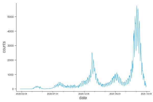
さて,最終段階である。欠損値を補間したデータフレーム df4 を使って,全期間のグラフを描画しよう。

  plot(df4.date, df4.counts,
  xlabel="date", xtickfontsize=6, tick_direction=:out, xminorticks=3, 
  ylabel="counts", size=(600, 400), grid=false, label="")

横軸目盛りのフォーマットを変更し,'年/月' にする。

  plot!(xformatter = x -> Dates.format(Date(Dates.UTD(x)), "yyyy/mm"))

VegaLite でも,適切な処理時間で,同じようなグラフが描ける。

  using VegaLite
  df4 |> @vlplot(
          mark=:line,
          x={:date, axis={grid=false, format="%Y-%b"}},
          y={:counts, axis={grid=false}},
          width=600,
          height=400)
コメント
  • X
  • Facebookでシェアする
  • はてなブックマークに追加する
  • LINEでシェアする

Julia で積み上げ棒グラフ,横軸が日付

2021年09月24日 | ブログラミング

以下に R/ggplot2 による積み上げ棒グラフの作成例がある
https://qiita.com/text_owleyes_0214/items/d6c815e04c284a5677a0

Julia だったらどんな風かな?

using CSV, DataFrames

# Julia では,直接は読めない
# dat = CSV.read("https://vrs-data.cio.go.jp/vaccination/opendata/latest/summary_by_date.csv", DataFrame)
# ArgumentError: "https://vrs-data.cio.go.jp/vaccination/opendata/latest/summary_by_date.csv" is not a valid file

#= 何回も直接読みに行くのは避けること

import Pkg; Pkg.add("HTTP") # まだインストールされていないなら
using HTTP
res = HTTP.get("https://vrs-data.cio.go.jp/vaccination/opendata/latest/summary_by_date.csv");
df = CSV.read(res.body, DataFrame);
rename!(df, [2 => :first, 3 => :second]);
CSV.write("vaccination.csv", df) # 読めたら保存しておく。
=#

df = CSV.read("vaccination.csv", DataFrame); # 二回目以降はこのファイルから入力する

using Plots, StatsPlots, Dates

Plots の groupedbar は,long format にする必要はない。
日付は月曜日の位置につける(文字列を斜めになんかしない)。
label が複数あるときは,1×n 列で指定する。
legend は枠外に出さない(出したければ legend=:outertopright)にする。

groupedbar(Matrix(df[[:first, :second]]), bar_position = :stack,
           bar_width=1, alpha=0.6,
           label=["first" "second"], legend=:topleft, # :outertopright,
           title = "Counts of vaccination, summary by date.",
           xlabel="date", ylabel="counts",
           xticks=(1:7:165, Dates.format.(df.date,"mm-dd")[1:7:165]),   
          
xtickfontsize=6, tick_direction=:out, yformatter=:plain,
          
grid=false, size=(800, 500))

ついでに,累積度数分布図も描いておく(というか,こちらの方が情報は多いか?)
まだ 2 回接種は,1 回接種の半分くらいなんだな。

df.cum_first = cumsum(df.first)
df.cum_second = cumsum(df.second);
groupedbar(Matrix(df[[:cum_first, :cum_second]]), bar_position = :stack, bar_width=1, alpha=0.6,
    label=["first" "second"], legend=:topleft, # :outertopright,
    title = "Cumulated counts of vaccination, summary by date.",
    xlabel="date", ylabel="cumulated counts",
    xticks=(1:7:165, Dates.format.(df.date,"mm-dd")[1:7:165]), xtickfontsize=6,
    tick_direction=:out, yformatter=:plain, grid=false, size=(800, 400))

VegaLite では,longformat にしないといけない(面倒じゃ)。

df2 = DataFrames.stack(df, 2:3);

rename!(df2, [:variable => :vaccined, :value => :counts]);

using VegaLite

記述は json ということで,馴染みがない。
legend は orient = "top-right" で。
VegaLite の 1 週間は日曜始まりのようだ。

df2 |>
       @vlplot(
           :bar,
           width = 600,
           height = 400,
           title = "Counts of vaccination, summary by date.",
           x = {:date, axis={format="%m-%d", title="date"}},
           y = :counts,
           color = {
               :vaccined,
               scale = {
                   domain = ["first", "second"],
                   range = ["#e7ba52a0", "#9467bda0"]
               },
               legend = {
                   title = "vaccined",
                   orient = "top-right"
               }
           },
           config = {
               axis = {
                   grid = false
               }
           }
       )

どちらでも,おなじくらい綺麗だ。ggplot2 には勝った。

コメント
  • X
  • Facebookでシェアする
  • はてなブックマークに追加する
  • LINEでシェアする

Julia の小ネタ--037 大小順や辞書順などではない,特別な順序に基づくソート

2021年09月16日 | ブログラミング

sort!() や sort() において,昇順とか降順は数値の大小とか文字列ならば辞書順(これも大小ではあるが)による。
しかし,ある場合には単なる辞書順ではなく別の基準で並べ替えなければならないことがある。
このような場合には,sort!() や sort() の引数の lt で関数を指定する。
その関数は引数を 2 つとり,a が b より前(昇順で b は a より後)ならば true,そうでなければ false を返す。デフォルトでは lt = isless である。isless も 2 つの引数をとり,例示するような結果を返す。

isless(1, 4) # true
isless("a", "abcde") # true
isless(π, ℯ) # π = 3.1415926535897...,ℯ = 2.7182818284590... ゆえ false

たとえば,年号が

nengou = ["明治", "大正", "昭和", "平成", "令和"]

のとき,普通にソートすると

sort(nengou)

#=
5-element Vector{String}:
 "令和"
 "大正"
 "平成"
 "明治"
 "昭和"
=#

になってしまう。

年号のデータを「"明治", "大正", "昭和", "平成", "令和"」の順でソートしたいときは以下のような関数を定義する。

function compare(a, b)
    rank(nengou) = indexin([nengou], ["明治", "大正", "昭和", "平成", "令和"])[1]
    return rank(a) <= rank(b)
end

そのうえで,

sort(nengou, lt=compare)

とすれば,以下の結果になる。

#=
5-element Vector{String}:
 "明治"
 "大正"
 "昭和"
 "平成"
 "令和"
=#

これは別に Julia だからということではなく,R でも Python でもそのような関数仕様になっている。

x = ["平成3", "令和2","大正7", "昭和6", "明治2", "令和1", "昭和9"]

のようなデータを年号と年の順に並べ替えるには,以下のような関数を使う。
年号を100の位,年を10, 1 の位に割り当てて一つの整数にして,大小関係を判定する関数である。
なお,データは UTF-8 なので,漢字の場合には文字数と桁数が異なるので注意が必要ではある。

function compare2(a, b)
    rank(nengou) = 100indexin([nengou[1:4]], ["明治", "大正", "昭和", "平成", "令和"])[1] + parse(Int, nengou[7:end])
    return rank(a) <= rank(b)
end

rank("明治23") # 123
rank("昭和5")  # 305

sort(x, lt=compare2)
#=
7-element Vector{String}:
 "明治2"
 "大正7"
 "昭和6"
 "昭和9"
 "平成3"
 "令和1"
 "令和2"
=#

コメント
  • X
  • Facebookでシェアする
  • はてなブックマークに追加する
  • LINEでシェアする

Julia の小ネタ--036 文字が文字列に含まれるか?

2021年09月16日 | ブログラミング

多くの言語では,1 文字が文字列中にあるかどうかは簡単な関数で調べることができる。

たとえば,Python なら

"abcdefg".find("c")   # 2
"abcdefg".find("z")   # -1 存在しない場合

Julia では,

occursin("c", "abcdefg")   # true
occursin("xyz", "abcdefg") # false

Julia の indexin(a, b) は a が b に含まれないときには nothing を返すという,ありがたいんだかありがたくないんだか,微妙な仕様になっている。

そこで,以下のような find 関数を実装してみた。

indexin() の a, b は配列でもよいのだけど,find() の第1引数は 文字型(Char)もしくは長さ1の文字列,第2引数は文字列または整数に限定する。引数の組み合わせとして4通りあるので,find() も 4 通り書き,最終的に5番目に定義する関数が呼ばれる。5番目の関数の第1引数は Char型,第2引数は Vector{Char} である。indexin() を呼び,結果が nothing のときには 0 を返すようにしている。

find(c::Char,   n::Int)     = find(c, string(n))
find(c::Char,   s::String)  = find(c, Char[s...])
find(s::String, n::Int)     = find(Char(s...), string(n))
find(s::String, ss::String) = find(Char(s...), Char[ss...])
function find(c::Char, cc::Vector{Char})
    x = indexin(c, cc)[1]
    isnothing.(x) ? 0 : x
end

この関数群がどのように働くかは実行例を見れば一目瞭然。

find('3', 123)   # 3
find('4', 123)   # 0
find('3', "123") # 3
find('4', "123") # 0
find("3", 123)   # 3
find("4", 123)   # 0
find("3", "123") # 3
find("4", "123") # 0


コメント
  • X
  • Facebookでシェアする
  • はてなブックマークに追加する
  • LINEでシェアする

Julia の小ネタ--035 文字列の append!

2021年09月15日 | ブログラミング

append!() により文字列を配列要素として追加するとき,以下のようにすると文字列が分解されて 1 文字ずつの Char 型で追加される。

a = []
append!(a, "12345")
a
#=
5-element Vector{Any}:
 '1': ASCII/Unicode U+0031 (category Nd: Number, decimal digit)
 '2': ASCII/Unicode U+0032 (category Nd: Number, decimal digit)
 '3': ASCII/Unicode U+0033 (category Nd: Number, decimal digit)
 '4': ASCII/Unicode U+0034 (category Nd: Number, decimal digit)
 '5': ASCII/Unicode U+0035 (category Nd: Number, decimal digit)
=#
typeof(a[1]) # Char

普通は,そうなることは望まない。文字列そのものを追加するときは,追加される文字列を配列として渡す。すなわち [ ] で囲む。

b = []
append!(b, ["12345"])
b
#=
1-element Vector{Any}:
 "12345"
=#
typeof(b[1]) # String

なぜ文字列一個なのに配列にしなければならないかというのは追加される文字列は 2 個以上でもよいからである。

上に引き続いてさらに 2 個の文字列を追加してみる。

append!(b, ["abc", "XYZ"])
b
#=
3-element Vector{Any}:
 "12345"
 "abc"
 "XYZ"
=#

コメント
  • X
  • Facebookでシェアする
  • はてなブックマークに追加する
  • LINEでシェアする

Julia で Python プログラムを動かす--その2

2021年09月12日 | ブログラミング

なにはともあれ,最初に using PyCall 追記あり(2021/09/13)

using PyCall

Python のパッケージの import は以下のようにする

math = pyimport("math") # import math as math に相当

パッケージ中の関数は Python で記述するそのまま

math.sin(math.pi / 4)  # 0.7071067811865475 # Python の math パッケージの sin と π
sin(pi / 4)            # 0.7071067811865475 Julia の sin 関数と π

np = pyimport("numpy") # import numpy as np に相当
np.arcsin(0.5)
arcsin(0.5)        # UndefVarError: arcsin not defined
                      
# Julia には arcsin という関数はないのでエラーになる
asin(0.5)              # 0.5235987755982989 # Julia では asin という名前
math.asin(0.5)         # 0.5235987755982988 # Python の math パッケージでは asin という名前

matplotlib.pyplot での描画

plt = pyimport("matplotlib.pyplot")
x = range(0;stop=2*pi,length=1000); # Julia で定義
y = sin.(3*x + 4*cos.(2*x));        # Julia で定義
plt.plot(x, y, color="red", linewidth=2.0, linestyle="--")
plt.show()

上のようにして PyPlot するのではなく,Julia で以下のようにすれば同じようにプロットできる(PyCall は明示的には使わない)。

using PyPlot
x = range(0;stop=2*pi,length=1000); # Julia で定義
y = sin.(3*x + 4*cos.(2*x));        # Julia で定義
plot(x, y, color="red", linewidth=2.0, linestyle="--")

あるライブラリをインポートしたときにエラーになるときの対処法

so = pyimport("scipy.optimize")

これを実行したとき,
    PyError (PyImport_ImportModule
    The Python package scipy.optimize could not be imported by pyimport.
と言われた場合は,scipy.optimize がないということである。
いつも使っている Python には scipy.optimize はあるのに?という場合は,エラーメッセージに示されているサジェスチョンに従う必要がある。

Julia が想定する Python は Conda.jl パッケージ でインストールされる最小限の Python(minimal Python distribution)である。そこには scipy.optimize はないということである。

いくつかある対処法のどれを採用するか迷うかも知れないが,もっとも適切なのは,通常使っている Python を使うことであろうか。その場合には,以下の 3 行に示すように PyCall を再ビルドする必要がある(Python のバージョンが変わった場合には常に再ビルドした方が良い)。

# ENV["PYTHON"] = "/usr/local/bin/python3"
# using Pkg
# Pkg.build("PyCall")

なお,元の Julia 依存の Python を使う場合は,1行目を ENV["PYTHON"] = "" として PyCall を再ビルドすればよい。

また,再ビルドした場合は,一度 Julia を終了し,再度 Julia を立ち上げる必要がある。

なにはともあれ,Python の scipy.optimize がインポートできれば,そのなかの newton 関数を使えると言うことである。

so.newton(x -> cos(x) - x, 1) # 0.7390851332151607

pycall で Python の関数を呼ぶ

pycall(func::PyObject, returntype::Type, args...)
@pycall func(args...)::returntype

math.sqrt(3.0)
pycall(math.sqrt, PyAny, 3.0)   # 1.7320508075688772
pycall(math.sqrt, Float64, 3.0) # 1.7320508075688772
@pycall math.sqrt(3.0)::Float64 # 1.7320508075688772

using Random; Random.seed!(12345)
x = randn(100);
sum(x)                   # 0.9821131440360702 Julia の sum 関数
pycall(np.sum, PyAny, x) # 0.9821131440360702 
np.sum(x)                # 0.9821131440360702

前の記事にも書いたが,py"...", py"""...""" で ... の部分に書かれた Python プログラムを実行できる。

using PyCall

py"""
import numpy as np
def f(x):
    return x**2
"""

py"f(5)" # 25

py"\"hello\"" # py"print(\"hello\")"

"""...""" は結果を返さない(後述)

py"print(\"hello\")"

py"""
print(9)
"""

Julia 中での変数などを PyCall で参照するのは「$変数名」でできる(RCall と同じ)。
また,PyCall の結果も,Julia の変数に代入できる。

using PyCall

以下の例は,Julia の配列 [1,2,3] を Python の sum 関数で和をとる例である。

py"sum($([1,2,3]))" # 6

配列 x を $x で参照する。

x = [1, 2, 3]
py"sum($x)" # 6

Julia の文字列変数は $y, $$y のようにして使用できる。

y = "1+2+3"

$y は文字列そのまま使用される

py"$y" # "1+2+3"

$$y は文字列を評価して使用される

py"$$y" # 6

直接文字列を記載する場合は \ でエスケープする。

py"$$(\"1+2+3\")" # 6

以下の例で,sqrt(8)+1 は Python の式として評価される。従って sqrt() という関数はないのでエラーになる。

z = "sqrt(8)+1"
py"$$z" # PyError

math パッケージをインポートしてもエラーになる。結局,解決法はまだわからない。

math = pyimport("math")

当然,以下は正しく実行される。

math.sqrt(8)+1 # 3.8284271247461903

z = "math.sqrt(8)+1" # "math.sqrt(8)+1"
py"$z" # "math.sqrt(8)+1"
py"$$z" # PyError

引き渡される文字列は「Python の式」であることに注意が必要。

以下は「2 の 4 乗から 3 を引く」つまり結果として 13 を得る。

z = "2**4-3"
py"$$z" # 13

以下は「2 と 4 のビット和から 3 を引く」。つまり 0b010 と 0b100 のビット和 0b110 = 6 から 3 を引くので,結果は 3 になる。

z = "2^4-3"
py"$$z" # 3

前にも述べたが,"""...""" は結果を返さない。

py"""
x = 2
y = 3
x ** y
"""

Julia に結果を返す変数を global 指定すると後で引用できる。

py"""
global g
x = 2
y = 3
g = x ** y
"""

py"g"     # 8
a = py"g" # 8
a         # 8


コメント
  • X
  • Facebookでシェアする
  • はてなブックマークに追加する
  • LINEでシェアする

家紋シリーズ 雁金(1) 丸に雁金

2021年09月11日 | ブログラミング

家紋シリーズ 雁金(1) 丸に雁金

これはもはや,自由曲線のみでの描画。

# plotter.jl を include
# https://blog.goo.ne.jp/r-de-r/e/bd71a52a09801335d56f7c47d879bfe3
# bezier 曲線の関数は,以前のプログラム例を参照

include("plotter.jl")

function karigane(; r=1, width=400, height=400)
    plotbegin(w=width, h=height)
    xy1 = bezier([550 709; 508 751; 476 776; 441 793; 399 814;
                  360 826; 328 834; 266 839; 165 835; 130 828;
                  88 811; 67 797; 46 786; 25 776; 0 762])
    xy2 = bezier([550 709; 522 709; 473 712; 413 709; 374 705;
                  339 698; 307 688; 272 673; 243 663; 215 645;
                  183 624; 148 596; 124 571; 99 539; 78 515;
                  53 476; 35 441; 14 398; 5 370])
    xy3 = [0 762; 0 356]
    x = vcat(xy1[:, 1], xy3[:, 1], reverse(xy2[:, 1]))
    y = vcat(xy1[:, 2], xy3[:, 2], reverse(xy2[:, 2]))
    plotpolygon(x , y, lwd=0, fcol=:black)
    plotpolygon(-x, y, lwd=0, fcol=:black)
    xy4 = vcat(bezier([0 1018; 46 1016; 81 1010; 106 985; 130 970;
                       148 949; 173 899; 176 846; 176 740]),
              [176 740; 0 740; 0 1030])
    plotpolygon(xy4[:, 1] , xy4[:, 2], lwd=0, fcol=:black)
    plotpolygon(-xy4[:, 1] , xy4[:, 2], lwd=0, fcol=:black)
    xy5 = bezier([172 826; 130 824; 88 808; 67 797; 46 788;
                  25 776; 0 762])
    plotline(xy5[:, 1], xy5[:, 2], lwd=2, col=:white)
    plotline(-xy5[:, 1], xy5[:, 2], lwd=2, col=:white)
    plotcircle(-46, 930, 26, lwd=1.7, col=:white)
    plotcircle(-46, 930, 12, col=:white, lwd=0, fcol=:white)
    xy6 = bezier([-71 853; -49 846; -39 839; -21 840; 3 850; 18 860;
                  28 874; 39 892; 39 910; 42 934])
    plotline(xy6[:, 1], xy6[:, 2], lwd=2, col=:white)
    plotpolygon([-247, -166, -154], [888, 904, 865],
                lwd=2, col=:white, fcol=:black)
    plotpolygon([-247, -154, -183], [888, 863, 831],
                lwd=2, col=:white, fcol=:black)
    plotring(0, 702, 702, 569)
    plotend()
end

karigane()

コメント
  • X
  • Facebookでシェアする
  • はてなブックマークに追加する
  • LINEでシェアする

Julia で Python プログラムを動かす

2021年09月11日 | ブログラミング

Julia で R を使う

https://blog.goo.ne.jp/r-de-r/e/4c859e73fd986d7da5b73c1991a81cfb
https://blog.goo.ne.jp/r-de-r/e/a9091dc91520c627d86bb799ee9f6f47

と同じように,Julia で Python  が使える。

using PyCall しておいて,トリプルクオートでくくったパイソンプログラムの前に py を付けるだけだ。一行だけの場合は py"プログラム" で実行される。

詳しくは

https://github.com/JuliaPy/PyCall.jl

Python にしかない関数を Julia で使うには便利かな。

using PyCall

py"""

import numpy as np
def f(x):
    return x**2
"""

py"f(5)"


コメント
  • X
  • Facebookでシェアする
  • はてなブックマークに追加する
  • LINEでシェアする

modulus は「絶対値」じゃない --- その後

2021年09月10日 | ブログラミング

modulus は「絶対値」じゃない
https://blog.goo.ne.jp/r-de-r/e/a6ddf31b879b083d6d62923310aec2ac

であるが,

要約すると

> 30284005485024840 %% 7
[1] 4

> 30284005485024840 %% 6
[1] 0
 警告メッセージ:
 絶対値で精度が完全に失われた可能性があります  

ということだったが,最近の R  では様相が違うようである。

事情により最新とは言えない R version 4.0.5 であるが,

> 30284005485024840 %% 7
[1] 3

> 30284005485024840 %% 6
[1] 0

最初の答えは 4 ではなく 3 であるし,

二番目の答えは 0 であるが,おかしなエラーメッセージは表示されない。

R 自身の多精度演算ライブラリの gmp でも確かめたが,

> library(gmp)

> as.bigz(30284005485024840) %% 7
Big Integer ('bigz') :
[1] 3

> as.bigz(30284005485024840) %% 6
Big Integer ('bigz') :
[1] 0

なので,今の状態が正しいようだ。

整数演算が自動的に多倍長で行われる Python でも

30284005485024840 % 7 # 3
30284005485024840 % 6 # 0

Julia でも

BigInt(30284005485024840) % 7 # 3
BigInt(30284005485024840) % 6 # 0

R の以前のざまは,何だったのか。

ということで,「 絶対値で精度が完全に失われた可能性があります 」という珍訳メッセージもお役御免と言うことだろうか。

コメント
  • X
  • Facebookでシェアする
  • はてなブックマークに追加する
  • LINEでシェアする

家紋シリーズ 片喰(2) 丸に剣片喰,角立て井筒に片喰,片喰

2021年09月10日 | ブログラミング

家紋シリーズ 片喰(2) 丸に剣片喰,角立て井筒に片喰,片喰

家紋シリーズ 片喰(1) 丸に角立て井筒に剣片喰 は片喰に丸と角立て井筒の装飾があるものだったので,装飾を除いたバージョンを描けるように引数を追加した。

function kenkatabami(; r=1, igeta=true, maru=true, width=400, height=400)
    plotbegin(w=width, h=height)
    for θ ∈ [0, 120, 240]
        ken(θ, r)
        katabami(θ, r)
        ken(θ, r, true)
        katabami(θ, r, true)
    end
    for θ ∈ [30, 150, 270]
        y, x = 70r .* sincosd(θ)
        plotline(0, 0, x, y, lwd=2, col=:white)
        plotcircle(x, y, 10r, lwd=0, col=:white, fcol=:white)
    end
    plotcircle(0, 0, 40r, lwd=0, col=:white, fcol=:white)
    plotcircle(0, 0, 30r, lwd=0, col=:black, fcol=:black)
    igeta && plotigeta(r)
    if igeta == maru == true
        plotring(0, 0, 700r, 580r)
    elseif maru
        plotring(0, 0, 260r, 300r)
    end
    plotend()
end

kenkatabami(igeta=false)

kenkatabami(maru=false)

kenkatabami(igeta=false, maru=false)

コメント
  • X
  • Facebookでシェアする
  • はてなブックマークに追加する
  • LINEでシェアする

家紋シリーズ 片喰(1) 丸に角立て井筒に剣片喰

2021年09月10日 | ブログラミング

家紋シリーズ 片喰(1) 丸に角立て井筒に剣片喰

自由曲線をベジェ曲線で近似する

# ベジェ曲線
function bezier(P; points=50)
    spline(P, size(P, 1) - 1; points)
end

function spline(P, n; points=50)
    # p = size(P, 1)  # Number of Control Ponits
    # n = 3           # Degree of B-Spline
    # n = p -1        # Bezier curve
    p = size(P, 1)
    m = p + n + 1     # Number of Knots in Knot Vector

    # Define Knot Vector
    u = OpenUniformKnotVector(m, n)
    # t = 0:0.01:u[end]
    # t = range()
    t = range(u[1], stop=u[end], length=points)

    # Calculate B-spline Curve
    S = zeros(length(t), 2);
    S[1, :] = P[1, :]
    for i ∈ 2:length(t)
        for j ∈ 1:p
            b = BasisFunction(u, j, n, t[i])
            S[i, :] += P[j, :] * b
        end
    end
    S
end

# u : Knot Vector
# m : Number of Knots in Knot Vector
# n : Degree of B-Spline
function OpenUniformKnotVector(m, n)
    u = zeros(1, m)
    for i ∈ 1:m
          if i < n+1
              u[i] = 0
          elseif i > m - (n + 1)
              u[i] = m - 1 - 2 * n
          else
              u[i] = i - n - 1
          end
    end
    u ./ u[end]
end

# u : Knot Vector
# j : j-th Control Ponit
# k : k-th Basis Function <-- n-th B-Spline
# t : Time
function BasisFunction(u, j, k, t)
    w1, w2 = 0, 0

    if k == 0
        if u[j] < t <= u[j+1]
            var = 1
        else
            var = 0
        end
    else
        if u[j+k+1] != u[j+1]
            w1 = BasisFunction(u, j+1, k-1, t) *
                              (u[j+k+1] - t)/(u[j+k+1]-u[j+1])
        end
        if u[j+k] != u[j]
            w2 = BasisFunction(u, j, k-1, t) *
                              (t - u[j])/(u[j+k] - u[j])
        end
        var = w1 + w2
    end
    var
end

# plotter.jl を include
# https://blog.goo.ne.jp/r-de-r/e/bd71a52a09801335d56f7c47d879bfe3

include("plotter.jl")

function ken(θ, r, mirror=false)
    t = [cosd(θ) sind(θ); -sind(θ) cosd(θ)]
    xy1 = r .* [-0.5 38; -0.5 251]
    xy2 = bezier(r .* [3 251; 25 232; 49 222; 77 219])
    xy2 = bezier(r .* [0 251; 25 232; 49 222; 77 219])
    xy3 = bezier(r .* [77 219; 53 180; 35 152; 21 117; 14 78; 10 60; 10 38])
    xy = vcat(xy1, xy2, xy3)
    if mirror
        xy[:, 1] = -xy[:, 1]
    end
    xy = xy * t
    plotpolygon(xy[:, 1], xy[:, 2], lwd=0, fcol=:black)
end

function katabami(θ, r, mirror=false)
    t = [cosd(θ) sind(θ); -sind(θ) cosd(θ)]
    xy1 = bezier(r .* [25 30; 26 67; 32 95; 42 131; 53 155; 66 176; 75 187; 90 198; 107 205; 125 205])
    xy2 = bezier(r .* [125 205; 141 205; 159 201; 169 191; 183 176; 194 162; 197 141; 198 109])
    xy3 = r .* [198 109; 39 21; 25 21]
    xy = vcat(xy1, xy2, xy3)
    if mirror
        xy[:, 1] = -xy[:, 1]
    end
    xy = xy * t
    plotpolygon(xy[:, 1], xy[:, 2], lwd=0, fcol=:black)
end

function igeta(r, θ)
    t = [cosd(θ) sind(θ); -sind(θ) cosd(θ)]
    xy = r .* [46 564; 116 494; -494 -116; -564 -46] * t
    plotpolygon(xy[:, 1], xy[:, 2], lwd=0, fcol=:black)
end

function plotigeta(r)
    for θ ∈ 0:90:270
        igeta(r, θ)
    end
end

function plotring(x, y, r1=1.0, r2=0.9; startθ=0, endθ=360, fcol=:black)
    r1, r2 = max(r1, r2), min(r1, r2)
    θ = startθ:endθ;
    coordx = cosd.(θ);
    coordy = sind.(θ);
    plotpolygon(x .+ vcat(r1 .* coordx, r2 .* reverse(coordx)), y .+ vcat(r1 .* coordy, r2 .* reverse(coordy)), col=fcol, lwd=0, fcol=fcol)
end

# メインプログラム
function kenkatabami(; r=1, width=400, height=400)
    plotbegin(w=width, h=height)
    for θ ∈ [0, 120, 240]
        ken(θ, r)
        katabami(θ, r)
        ken(θ, r, true)
        katabami(θ, r, true)
    end
    for θ ∈ [30, 150, 270]
        y, x = 70r .* sincosd(θ)
        plotline(0, 0, x, y, lwd=2, col=:white)
        plotcircle(x, y, 10r, lwd=0, col=:white, fcol=:white)
    end
    plotcircle(0, 0, 40r, lwd=0, col=:white, fcol=:white)
    plotcircle(0, 0, 30r, lwd=0, col=:black, fcol=:black)
    plotigeta(r)
    plotring(0, 0, 700r, 580r)
    plotend()
end

kenkatabami()


コメント
  • X
  • Facebookでシェアする
  • はてなブックマークに追加する
  • LINEでシェアする

家紋シリーズ 三つ兎

2021年09月09日 | ブログラミング

家紋シリーズ 三つ兎

自由曲線をベジェ曲線で近似する

# ベジェ曲線
# https://tajimarobotics.com/basis-spline-interpolation-program-2/

function bezier(P; points=50)
    spline(P, size(P, 1) - 1; points)
end

function spline(P, n; points=50)
    # p = size(P, 1)  # Number of Control Ponits
    # n = 3           # Degree of B-Spline
    # n = p -1        # Bezier curve
    p = size(P, 1)
    m = p + n + 1     # Number of Knots in Knot Vector

    # Define Knot Vector
    u = OpenUniformKnotVector(m, n)
    # t = 0:0.01:u[end]
    # t = range()
    t = range(u[1], stop=u[end], length=points)

    # Calculate B-spline Curve
    S = zeros(length(t), 2);
    S[1, :] = P[1, :]
    for i ∈ 2:length(t)
        for j ∈ 1:p
            b = BasisFunction(u, j, n, t[i])
            S[i, :] += P[j, :] * b
        end
    end
    S
end

# u : Knot Vector
# m : Number of Knots in Knot Vector
# n : Degree of B-Spline
function OpenUniformKnotVector(m, n)
    u = zeros(1, m)
    for i ∈ 1:m
          if i < n+1
              u[i] = 0
          elseif i > m - (n + 1)
              u[i] = m - 1 - 2 * n
          else
              u[i] = i - n - 1
          end
    end
    u ./ u[end]
end

# u : Knot Vector
# j : j-th Control Ponit
# k : k-th Basis Function <-- n-th B-Spline
# t : Time
function BasisFunction(u, j, k, t)
    w1, w2 = 0, 0

    if k == 0
        if u[j] < t <= u[j+1]
            var = 1
        else
            var = 0
        end
    else
        if u[j+k+1] != u[j+1]
            w1 = BasisFunction(u, j+1, k-1, t) *
                              (u[j+k+1] - t)/(u[j+k+1]-u[j+1])
        end
        if u[j+k] != u[j]
            w2 = BasisFunction(u, j, k-1, t) *
                              (t - u[j])/(u[j+k] - u[j])
        end
        var = w1 + w2
    end
    var
end

# plotter.jl を include
# https://blog.goo.ne.jp/r-de-r/e/bd71a52a09801335d56f7c47d879bfe3

include("plotter.jl")

function plotwhitecurve(ox, oy, r, t, xy)
    xy = bezier(xy)
    plotwhiteline(ox, oy, r, t, xy)
end

function plotwhiteline(ox, oy, r, t, xy)
    xy2 = r .* xy * t
    plotline(ox .+ xy2[:,1], oy .+ xy2[:, 2], col=:white, lwd=2)
    xy2 = xy; xy2[:, 1] *= -1
    xy2 = r .* xy * t
    plotline(ox .+ xy2[:,1], oy .+ xy2[:, 2], col=:white, lwd=2)
end

function ploteyes(ox, oy, r, t, xy, radius, color)
    xy2 = r .* xy *t
    for i ∈ 1:3
        plotcircle(ox + xy2[i, 1], oy + xy2[i, 2],
                   radius[i], lwd=0, fcol=color[i])
    end
    xy2 = xy; xy2[:, 1] *= -1
    xy2 = r .* xy *t
    for i ∈ 1:3
        plotcircle(ox + xy2[i, 1], oy + xy2[i, 2],
                   radius[i], lwd=0, fcol=color[i])
    end
end

function plothead(ox, oy, r, t)
    # 頭
    xy = bezier([0 692; 36 661; 67 633; 81 626; 138 597;
                 232 576; 237 580; 290 550; 342 530; 392 440]);
    # 耳(上)
    xy = vcat(xy, bezier([250 400; 388 425; 395 440; 392 445;
                          484 430; 494 400; 589 347]));
    # 耳(下)
    xy = vcat(xy, bezier([589 347; 500 290; 426 260; 250 270]));
    # 頬
    xy = vcat(xy, bezier([427 273; 395 157; 346 104; 272 61;
                          188 50; 159 22; 89 22; 5 5; 0 8]));
    xy2 = r .* xy * t
    plotpolygon(ox .+ xy2[:,1], oy .+ xy2[:, 2],
                lwd=0.5, col=:black, fcol=:black)
    xy2 = xy; xy2[:, 1] *= -1
    xy2 = r .* xy2 * t
    plotpolygon(ox .+ xy2[:,1], oy .+ xy2[:, 2],
                lwd=0.5, col=:black, fcol=:black)
end

function usagi1(R, r, θ)
    ox, oy = R * cosd(θ), R * sind(θ)
    θ += 90
    t = [cosd(θ) sind(θ); -sind(θ) cosd(θ)]
    plothead(ox, oy, r, t)
    # おでこ
    plotwhitecurve(ox, oy, r, t,
        [144 363; 112 394; 84 398; 53 412; 0 412])
    # 耳上白線
    plotwhitecurve(ox, oy, r, t,
        [96 329; 131 348; 159 365; 191 379; 230 394; 263 410;
        310 423; 352 435; 382 437; 422 437; 456 431; 489 418])
    # 耳下白線
    plotwhitecurve(ox, oy, r, t,
        [143 269; 145 269; 177 280; 198 286; 226 286; 254 273;
        297 265; 350 258; 392 265; 424 268; 452 274])
    # 目
    ploteyes(ox, oy, r, t,
        [74 216; 73 215; 72 214],
        [32, 22, 12], [:white, :black, :white])
    # 鬚
    plotwhiteline(ox, oy, r, t,
        [89 174; 191 220; NaN NaN; 81 160; 244 178; NaN NaN;
        74 142; 205 142])
    # 鼻
    plotwhitecurve(ox, oy, r, t,
        [-7 104; 0 100; 21 111; 18 125; 17 139; 36 157])
    # 上唇
    plotwhitecurve(ox, oy, r, t,
        [14 114; 32 100; 43 93; 57 90; 74 93; 89 100; 106 107])
    # 下唇
    plotwhitecurve(ox, oy, r, t,
        [0 68; 14 67; 29 75; 36 79; 43 93])
    # 頬
    plotwhitecurve(ox, oy, r, t,
        [99 8; 106 45; 117 60; 131 72; 149 86; 157 89; 180 97])
    # 足
    plotwhiteline(ox, oy, r, t,
        [134 15; 134 44; NaN NaN; 170 26; 170 44])
end

# メインプログラム
function usagi(; r=1, width=400, height=400)
    plotbegin(w=width, h=height)
    R = 725
    for θ ∈ [-30, 90, 210]
        usagi1(R, r, θ)
    end
    #usagi1(r, -0)
    plotend()
end

usagi()

savefig("fig.png")

コメント
  • X
  • Facebookでシェアする
  • はてなブックマークに追加する
  • LINEでシェアする

家紋シリーズ 輪違い(2) 丸に輪違い

2021年09月08日 | ブログラミング

# 家紋シリーズ 輪違い(2) 丸に輪違い

plotter.jl を include
https://blog.goo.ne.jp/r-de-r/e/bd71a52a09801335d56f7c47d879bfe3

include("plotter.jl")

# 塗りつぶしリングを描く
function plotring(x, y, r1=1.0, r2=0.9; startangle=0, endangle=360, fcol=:black)
    r1, r2 = max(r1, r2), min(r1, r2)
    θ = startangle:endangle;
    coordx = cosd.(θ);
    coordy = sind.(θ);
    plotpolygon(x .+ vcat(r1 .* coordx, r2 .* reverse(coordx)), y .+ vcat(r1 .* coordy, r2 .* reverse(coordy)), col=fcol, lwd=0, fcol=fcol)
end

function maruniwatigai(; r=1, r1=1.25r, r2 = 0.95r, width=400, height=400)
    plotbegin(w=width, h=height)
    plotring(0, 0, 2.2*r, 1.8*r, fcol=:black)
    plotring( 0.5r, 0, r1, r2, fcol=:black)
    plotring(-0.5r, 0, r1, r2, fcol=:black)
    plotring( 0.5r, 0, r1+0.03r, r1, startangle=110, endangle=150, fcol=:white)
    plotring( 0.5r, 0, r2-0.03r, r2, startangle= 90, endangle=130, fcol=:white)
    plotring(-0.5r, 0, r1+0.03r, r1, startangle=290, endangle=330, fcol=:white)
    plotring(-0.5r, 0, r2-0.03r, r2, startangle=270, endangle=310, fcol=:white)
    plotend()
end

maruniwatigai()

コメント
  • X
  • Facebookでシェアする
  • はてなブックマークに追加する
  • LINEでシェアする

家紋シリーズ 輪違い(1) 丸に三輪違い

2021年09月08日 | ブログラミング

# 家紋シリーズ 輪違い(1) 丸に三輪違い

plotter.jl を include
https://blog.goo.ne.jp/r-de-r/e/bd71a52a09801335d56f7c47d879bfe3

include("plotter.jl")

# 塗りつぶしリングを描く
function plotring(x, y, r1=1.0, r2=0.9; startangle=0, endangle=360, fcol=:black)
    r1, r2 = max(r1, r2), min(r1, r2)
    θ = startangle:endangle;
    coordx = cosd.(θ);
    coordy = sind.(θ);
    plotpolygon(x .+ vcat(r1 .* coordx, r2 .* reverse(coordx)), y .+ vcat(r1 .* coordy, r2 .* reverse(coordy)), col=fcol, lwd=0, fcol=fcol)
end

function marunimituwawatigai(; r=1,  r1=1.5r, r2 = 1.15r, width=400, height=400)
    plotbegin(w=width, h=height)
    plotring(0, 0, 102//35*r, 90/35*r, fcol=:black)
    for θ in -30:120:210
        centerx = r*cosd(θ)
        centery = r*sind(θ)
        plotring(centerx, centery, r1, r2, fcol=:black)
    end
    for θ in -30:120:210
        centerx = r*cosd(θ)
        centery = r*sind(θ)
        plotring(centerx, centery, r1+0.05r, r1, startangle= 80+θ, endangle=140+θ, fcol=:white)
        plotring(centerx, centery, r2, r2-0.05r, startangle= 80+θ, endangle=140+θ, fcol=:white)
        plotring(centerx, centery, r1+0.05r, r1, startangle=180+θ, endangle=240+θ, fcol=:white)
        plotring(centerx, centery, r2, r2-0.05r, startangle=180+θ, endangle=240+θ, fcol=:white)
    end
    plotend()
end

marunimituwawatigai()

コメント
  • X
  • Facebookでシェアする
  • はてなブックマークに追加する
  • LINEでシェアする

家紋シリーズ 稲妻(2) 角立て絡み稲妻

2021年09月04日 | ブログラミング

家紋シリーズ 稲妻(2) 角立て絡み稲妻

plotter.jl を include
https://blog.goo.ne.jp/r-de-r/e/bd71a52a09801335d56f7c47d879bfe3

include("plotter.jl")

function sumitatekaramiinazuma(; r=1, width=400, height=400)
    plotbegin(w=width, h=height)
    x = [0, 39, 5, -29, -5, 19, 5, -9, -5, 5, 11, -5,
         -21, 5, 31, -4] .* r

    y = [-39, 0, 34, 0, -24, 0, 14, 0, -4, 6, 0, -16,
         0, 26, 0, -35] .* r

    plotpolygon(x, y, lwd=0, fcol=:black)
    plotpolygon(-x , -y, lwd=0, fcol=:black)
    plotend()
end

sumitatekaramiinazuma()

コメント
  • X
  • Facebookでシェアする
  • はてなブックマークに追加する
  • LINEでシェアする

PVアクセスランキング にほんブログ村

PVアクセスランキング にほんブログ村