#==========
Julia の修行をするときに,いろいろなプログラムを書き換えるのは有効な方法だ。
以下のプログラムを Julia に翻訳してみる。
数量化 II 類
http://aoki2.si.gunma-u.ac.jp/R/qt2.html
ファイル名: qt2.jl 関数名: qt2, printqt2, plotqt2
翻訳するときに書いたメモ
カテゴリーデータのまま入力できるようにしようかとも思ったが,止めた。
==========#
using StatsBase, LinearAlgebra, Rmath, NamedArrays, Plots, StatsPlots
function qt2(dat, group; vname=[], cname=[], gname=[])
na = NamedArray
function geneig(a, b)
if size(a, 1) == 1
return a / b, 1
else
values, vectors = eigen(b, sortby=x-> -x)
g = Diagonal(1 ./ sqrt.(values))
v = vectors
values, vectors = eigen(g * v' * a * v * g, sortby=x-> -x)
vectors = v * g * vectors
return values, vectors
end
end
nc, item = size(dat)
index, n = table(group)
ng = length(n)
dat = hcat(dat, group)
cat = vec(maximum(dat, dims=1))
length(vname) > 0 || (vname = ["x$i" for i = 1:item])
length(gname) > 0 || (gname = ["g$i" for i = 1:ng])
if length(cname) == 0
cname = []
for i = 1:item
append!(cname, ["$(vname[i]).$j" for j = 1:cat[i]])
end
end
junjo = vcat(0, cumsum(cat)[1:end-1])
nobe2 = sum(cat)
nobe = nobe2 - ng
dat2 = zeros(Int, nc, nobe2)
for i = 1:nc
x0 = []
for j = 1:item + 1
zeros0 = zeros(cat[j])
zeros0[dat[i, j]] = 1
append!(x0, zeros0)
end
dat2[i, :] = x0
end
a2 = zeros(Int, nobe2, nobe2, nc)
for j = 1:nc
a2[:, :, j] = dat2[j, :] .* dat2[j, :]'
end
x = sum(a2, dims=3)
pcros = x[1:nobe, 1:nobe]
gcros = x[(nobe + 1):nobe2, 1:nobe]
w = (n * n') ./ nc
[w[i, i] = 0 for i = 1:ng]
grgr = Diagonal(n .- n .^ 2 / nc) - w
w = diag(pcros)
grpat = gcros - (n .* w') / nc
pat = pcros - (w .* w') / nc
select = (junjo .+ 1)[1:item]
suf = trues(nobe)
suf[select] .= false
pat = pat[suf, suf]
grpat = grpat[2:end, suf]
r = grgr[2:end, 2:end]
ndim = ng - 1
axisname = ["Axis-$i" for i = 1:ndim]
m = size(pat, 2)
c = grpat * (pat \ grpat')
values, vectors = geneig(c, r)
w = sqrt.(values)' .\ (pat \ grpat' * vectors)
a = zeros(nobe, ndim)
ie = 0
for j in 1:item
is = ie + 1
ie = is + cat[j] - 2
offset = junjo[j] + 2
a[offset:(offset + ie - is), :] = w[is:ie, :]
end
w = diag(pcros) .* a
for j in 1:item
is = junjo[j] + 1
ie = is + cat[j] - 1
s = sum(w[is:ie, :], dims=1) / nc
a[is:ie, :] = a[is:ie, :] .- s
end
a = sqrt.(diag(a' * pcros * a) ./ nc)' .\ a
samplescore = dat2[:, 1:nobe] * a
centroid = n .* vcat(0, vectors)
centroid = vcat(0, vectors) .- sum(centroid, dims=1) / nc
centroid = sqrt.(vec(sum(centroid .^ 2 .* n, dims=1)) ./ nc ./ values)' .\ centroid
item1 = item + 1
partialcorr = zeros(item, ndim)
for l = 1:ndim
pat = zeros(item1, item1)
pat[1, 1] = sum(n .* centroid[:, l] .^ 2)
temp = sum(a[:, l] .* transpose(gcros .* centroid[:, l]), dims=2)
is = junjo[1:end-1]
ie = junjo[1:end-1] + cat[1:end-1]
pat[1, 2:(item + 1)] = [sum(temp[is[k]+1:ie[k]]) for k = 1:length(is)]
temp = (a[:, l] * a[:, l]') .* pcros
for i = 1:item
is = junjo[i] + 1
ie = is + cat[i] - 1
for j = 1:i
pat[j + 1, i + 1] = sum(temp[is:ie, (junjo[j] + 1):(junjo[j] + cat[j])])
end
end
d = diag(pat)
pat = pat ./ sqrt.(d * d')
pat = pat + transpose(pat)
[pat[i, i] = 1 for i = 1:item1]
pat = inv(pat)
partialcorr[:, l] = -pat[2:item1, 1] ./ sqrt.(pat[1, 1] * diag(pat)[2:item1])
end
Dict(:nc => nc, :ndim => ndim, :group => group, :ng => ng, :categoryscore => a,
:partialcorr => partialcorr, :centroid => centroid, :eta => values,
:samplescore => samplescore, :vname => vname, :gname => gname,
:cname => cname, :axisname => axisname)
end
function table(x) # indices が少ないとき
indices = sort(unique(x))
counts = zeros(Int, length(indices))
for i in indexin(x, indices)
counts[i] += 1
end
return indices, counts
end
function table(x, y) # 二次元
indicesx = sort(unique(x))
indicesy = sort(unique(y))
counts = zeros(Int, length(indicesx), length(indicesy))
for (i, j) in zip(indexin(x, indicesx), indexin(y, indicesy))
counts[i, j] += 1
end
return indicesx, indicesy, counts
end
function printqt2(obj)
axisname = obj[:axisname]
println("\ncategory score\n", NamedArray(obj[:categoryscore], (obj[:cname], axisname)))
println("\npartial correlation coefficient\n", NamedArray(obj[:partialcorr], (obj[:vname], axisname)))
println("\nsample score\n", NamedArray(obj[:samplescore], (1:obj[:nc], axisname)))
println("\ncentroids\n", NamedArray(obj[:centroid], (obj[:gname], axisname)))
println("\neta\n", NamedArray(reshape(obj[:eta], 1, :), (["eta"], axisname)))
end
function plotqt2(obj; i = 1, j = 2, color=:blue, nclass = 20, which = "boxplot") # or "barplot" or "categoryscore"
pyplot()
if which == "categoryscore"
categoryscore = obj[:categoryscore][end:-1:1, i]
cname = [" $s " for s in obj[:cname][end:-1:1]]
align = [c > 0 ? :right : :left for c in categoryscore]
plt = bar(categoryscore, orientation=:h, grid=false,
yshowaxis=false, yticks=false,
xlabel=which, label="")
annotate!.(0, 1:length(cname), text.(cname, align, 8))
vline!([0], color=:black, label="")
else
group = obj[:group]
if obj[:ndim] > 1
xlabel, ylabel = obj[:axisname][[i, j]]
grouplevels = obj[:gname]
samplescore = obj[:samplescore]
plt = scatter(samplescore[:, i], samplescore[:, j], grid=false,
tick_direction = :out, xlabel = xlabel,
ylabel = ylabel, color = color, markerstrokecolor=color,
label="")
else
if which == "boxplot"
plt = boxplot(obj[:gname], obj[:samplescore][:, 1], grid=false,
tick_direction = :out, xlabel = "group",
ylabel = "sample score", label="")
elseif which == "barplot"
samplescore = obj[:samplescore][:, 1];
minx, maxx = extrema(samplescore)
w = (maxx - minx) / (nclass - 1)
samplescore2 = floor.(Int, (samplescore .- minx) ./ w)
index1, index2, res = table(samplescore2, group)
plt = groupedbar(res, xlabel = "sample score", label="")
end
end
end
display(plt)
end
dat = [
3 2
3 1
3 2
2 1
2 1
3 1
2 1
1 2]
group = [1, 2, 2, 1, 2, 2, 1, 2]
obj = qt2(dat, group)
printqt2(obj)
#=====
category score
5×1 Named Matrix{Float64}
A ╲ B │ Axis-1
──────┼─────────
x1.1 │ 2.31046
x1.2 │ -1.61032
x1.3 │ 0.630126
x2.1 │ 0.630126
x2.2 │ -1.05021
partial correlation coefficient
2×1 Named Matrix{Float64}
A ╲ B │ Axis-1
──────┼─────────
x1 │ 0.612372
x2 │ 0.421464
sample score
8×1 Named Matrix{Float64}
A ╲ B │ Axis-1
──────┼──────────
1 │ -0.420084
2 │ 1.26025
3 │ -0.420084
4 │ -0.980196
5 │ -0.980196
6 │ 1.26025
7 │ -0.980196
8 │ 1.26025
centroids
2×1 Named Matrix{Float64}
A ╲ B │ Axis-1
──────┼──────────
g1 │ -0.793492
g2 │ 0.476095
eta
1×1 Named Matrix{Float64}
A ╲ B │ Axis-1
──────┼─────────
eta │ 0.377778
=====#
x1 = [3, 3, 3, 2, 2, 3, 2, 1];
x2 = [2, 1, 2, 1, 1, 1, 1, 2];
group = [1, 2, 2, 1, 2, 3, 3, 3];
dat = hcat(x1, x2);
obj = qt2(dat, group)
printqt2(obj)
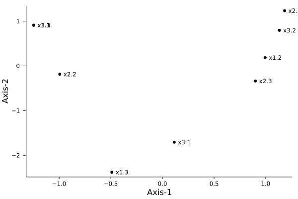
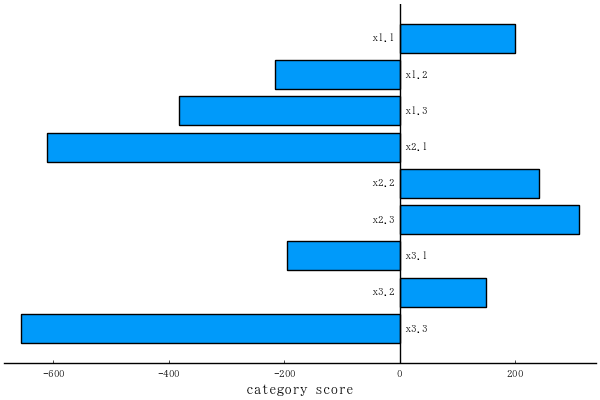
#=====
category score
5×2 Named Matrix{Float64}
A ╲ B │ Axis-1 Axis-2
──────┼───────────────────────
x1.1 │ 3.14099 0.267697
x1.2 │ -0.917694 1.19527
x1.3 │ -0.0969778 -0.963377
x2.1 │ 0.712515 -0.655608
x2.2 │ -1.18752 1.09268
partial correlation coefficient
2×2 Named Matrix{Float64}
A ╲ B │ Axis-1 Axis-2
──────┼───────────────────
x1 │ 0.630249 0.239844
x2 │ 0.513893 0.203824
sample score
8×2 Named Matrix{Float64}
A ╲ B │ Axis-1 Axis-2
──────┼─────────────────────
1 │ -1.2845 0.129304
2 │ 0.615537 -1.61899
3 │ -1.2845 0.129304
4 │ -0.205179 0.539662
5 │ -0.205179 0.539662
6 │ 0.615537 -1.61899
7 │ -0.205179 0.539662
8 │ 1.95347 1.36038
centroids
3×2 Named Matrix{Float64}
A ╲ B │ Axis-1 Axis-2
──────┼─────────────────────
g1 │ -0.744841 0.334483
g2 │ -0.291382 -0.316673
g3 │ 0.787942 0.0936848
eta
1×2 Named Matrix{Float64}
A ╲ B │ Axis-1 Axis-2
──────┼─────────────────────
eta │ 0.403355 0.0688667
=====#
plotqt2(obj)
plotqt2(obj, which="barplot")
plotqt2(obj, which="categoryscore") # savefig("fig1.png")
 using RDatasets
iris = dataset("datasets", "iris");
data = Matrix(iris[:, 1:4]);
group = vcat(repeat([1], 50), repeat([2], 50), repeat([3], 50)...);
for i = 1:4
q = quantile(data[:, i])
for k = 1:150
x = data[k, i]
for j = 2:5
if x <= q[j]
data[k, i] = j-1
break
end
end
end
end
obj = qt2(Int.(data), group)
color = vcat(repeat([:blue], 50), repeat([:black], 50), repeat([:red], 50)...);
plotqt2(obj, color=color) # savefig("fig2.png")
using RDatasets
iris = dataset("datasets", "iris");
data = Matrix(iris[:, 1:4]);
group = vcat(repeat([1], 50), repeat([2], 50), repeat([3], 50)...);
for i = 1:4
q = quantile(data[:, i])
for k = 1:150
x = data[k, i]
for j = 2:5
if x <= q[j]
data[k, i] = j-1
break
end
end
end
end
obj = qt2(Int.(data), group)
color = vcat(repeat([:blue], 50), repeat([:black], 50), repeat([:red], 50)...);
plotqt2(obj, color=color) # savefig("fig2.png")