【R前処理講座19】{dplyr} group_by:グルーピング【tidyverse】
https://datasciencemore.com/dplyr-group-by/
以下のようなデータフレームにおいて,グループごとの基礎統計量を求める。
まずは 1 変数でグループ化する場合。
using RCall
R"""
library(dplyr)
# define dataframe
df =
tibble(
class = c("a", "b", "c", "c", "a", "c", "b", "a", "c", "b", "a", "x"),
gender = c("M", "F", "F", "M", "F", "M", "M", "F", "M", "M", "F", "F"),
height = c(162, 150, 168, 173, 162, 198, 182, 154, 175, 160, 172, 157)
)
"""
#=
RObject{VecSxp}
# A tibble: 12 x 3
class gender height
1 a M 162
2 b F 150
3 c F 168
4 c M 173
5 a F 162
6 c M 198
7 b M 182
8 a F 154
9 c M 175
10 b M 160
11 a F 172
12 x F 157
=#
まずは class ごとに height の平均値を求める。
R でやると以下のようになる。
パイプの最後を print.data.frame にしているのは,結果が tibble で,それをデフォルトの print.tbl_df が使われてしまい小数点以下の桁数の表示に支障をきたすので,data.frame として出力するためである。
R"""
df %>%
group_by(class) %>%
summarise(mean = mean(height)) %>%
print.data.frame
""";
#=
class mean
1 a 162.5
2 b 164.0
3 c 178.5
4 x 157.0
=#
Julia でやってみよう。
using DataFrames
df = DataFrame(class = ["a", "b", "c", "c", "a", "c", "b", "a", "c", "b", "a", "x"],
gender = ["M", "F", "F", "M", "F", "M", "M", "F", "M", "M", "F", "F"],
height = [162, 150, 168, 173, 162, 198, 182, 154, 175, 160, 172, 157]
);
やり方は何通りかある。
グループ化 groupby() と combine() を 分ける書き方。
最後の |> println は表示形式を若干簡単にするためのものなので,REPL の場合はなくてもよい。
using Statistics
gdf = groupby(df, :class);
combine(gdf, :height=>mean=>:mean) |> println
#=
4×2 DataFrame
Row │ class mean
│ String Float64
─────┼─────────────────
1 │ a 162.5
2 │ b 164.0
3 │ c 178.5
4 │ x 157.0
=#
関数を入れ子にする書き方。出力は同じなので省略。
combine(groupby(df, :class), :height=>mean=>:mean) |> println
パイプを使う書き方。
groupby(df, :class) |> x -> combine(x, :height=>mean=>:mean) |> println
@chain マクロを使う書き方。
using DataFramesMeta # Chain もエクスポートされる
@chain df begin
groupby(:class)
combine(:height=>mean=>:mean)
println
end
複数の変数でグループ化して基本統計量を求める。
まずは R の場合
R"""
df %>%
group_by(class, gender) %>%
summarise(mean = mean(height), .groups="keep") %>%
print.data.frame
""";
#=
class gender mean
1 a F 162.6667
2 a M 162.0000
3 b F 150.0000
4 b M 171.0000
5 c F 168.0000
6 c M 182.0000
7 x F 157.0000
=#
Julia では,何通りかの書き方がある。
関数を入れ子にする書き方。
println(sort(combine(groupby(df, [:class, :gender]), :height=>mean=>:mean)))
#=
7×3 DataFrame
Row │ class gender mean
│ String String Float64
─────┼─────────────────────────
1 │ a F 162.667
2 │ a M 162.0
3 │ b F 150.0
4 │ b M 171.0
5 │ c F 168.0
6 │ c M 182.0
7 │ x F 157.0
=#
パイプを使う書き方。
groupby(df, [:class, :gender]) |> x -> combine(x, :height=>mean=>:mean) |> sort |> println
@chain マクロを使う書き方。
@chain df begin
groupby([:class, :gender])
combine(:height=>mean=>:mean)
sort
println
end
ところで,今までの出力例はちょっとわかりにくい。
以下のようにすれば,表形式で表示できる。このようにすることにより,存在しない組み合わせがあることに気づくことができる。つまり,class = "x", gender = "M" は存在しないということである。セルには missing が表示される。
aggregate = sort(combine(groupby(df, [:class, :gender]), :height=>mean=>:mean));
unstack(aggregate, :class, :gender, :mean) |> println
#=
4×3 DataFrame
Row │ class F M
│ String Float64? Float64?
─────┼─────────────────────────────
1 │ a 162.667 162.0
2 │ b 150.0 171.0
3 │ c 168.0 182.0
4 │ x 157.0 missing
=#
度数も求めることができる。
aggregate2 = sort(combine(groupby(df, [:class, :gender]), :height=>length=>:n));
unstack(aggregate2, :class, :gender, :n) |> println
#=
4×3 DataFrame
Row │ class F M
│ String Int64? Int64?
─────┼─────────────────────────
1 │ a 3 1
2 │ b 1 2
3 │ c 1 3
4 │ x 1 missing
=#
なお,度数の場合は FreqTables::freqtable() で求めるのが簡単である。
using FreqTables
freqtable(df, :class, :gender)
#=
4×2 Named Matrix{Int64}
class ╲ gender │ F M
───────────────┼─────
a │ 3 1
b │ 1 2
c │ 1 3
x │ 1 0
=#
平均値以外の基本統計量を求める。
まずは,R で。
R"""
df %>%
group_by(class) %>%
summarise(
Max = max(height),
Q3 = quantile(height, 0.75),
Mean = mean(height),
Median = median(height),
Q1 = quantile(height, 0.25),
Min = min(height),
sd = sd(height),
n = n()
) %>%
print.data.frame
""";
#=
class Max Q3 Mean Median Q1 Min sd n
1 a 172 164.50 162.5 162 160.00 154 7.371115 4
2 b 182 171.00 164.0 160 155.00 150 16.370706 3
3 c 198 180.75 178.5 174 171.75 168 13.329166 4
4 x 157 157.00 157.0 157 157.00 157 NA 1
=#
Julia もほぼ同じ程度の書き方でできる。
@chain df begin
groupby(:class)
@combine begin
:Max = maximum(:height)
:Q3 = quantile(:height, 0.75)
:Mean = mean(:height)
:Median = median(:height)
:Q1 = quantile(:height, 0.25)
:Min = minimum(:height)
:SD = std(:height)
:n = length(:height)
end
println
end
#=
4×9 DataFrame
Row │ class Max Q3 Mean Median Q1 Min SD n
│ String Int64 Float64 Float64 Float64 Float64 Int64 Float64 Int64
─────┼────────────────────────────────────────────────────────────────────────────
1 │ a 172 164.5 162.5 162.0 160.0 154 7.37111 4
2 │ b 182 171.0 164.0 160.0 155.0 150 16.3707 3
3 │ c 198 180.75 178.5 174.0 171.75 168 13.3292 4
4 │ x 157 157.0 157.0 157.0 157.0 157 NaN 1
=#
上の @chain マクロを使った書き方は,以下のように展開される。
以下を実行すれば,同じ結果が得られる。
combine(groupby(df, :class),
:height => maximum => :Max,
:height => (x -> quantile(x, 0.75)) => :Q3,
:height => mean => :Mean,
:height => median => :Median,
:height => (x -> quantile(x, 0.25)) => :Q1,
:height => minimum => :Min,
:height => std => :SD,
nrow => :n
) |> println
combine() は,以下のようにまとめて書くこともできる。
combine(groupby(df, :class),
fill(:height, 8) .=>
[maximum, (x -> quantile(x, 0.75)), mean, median,
(x -> quantile(x, 0.25)), minimum, std, length] .=>
[:Max, :Q3, :Mean, :Median, :Q1, :Min, :SD, :n]) |> println
この記法を用いて,すべての変数についての基礎統計料を得ることができる。
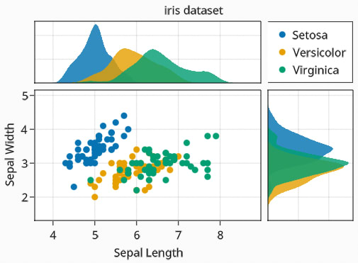
using DataFrames, RDatasets
iris = dataset("datasets", "iris");
for i in [:SepalLength, :SepalWidth, :PetalLength, :PetalWidth]
println("\nStatistic of $i")
combine(groupby(iris, :Species),
i => maximum => :Max,
i => (x -> quantile(x, 0.75)) => :Q3,
i => mean => :Mean,
i => median => :Median,
i => (x -> quantile(x, 0.25)) => :Q1,
i => minimum => :Min,
i => std => :SD,
nrow => :n
) |> println
end
#=
Statistic of SepalLength
3×9 DataFrame
Row │ Species Max Q3 Mean Median Q1 Min SD n
│ Cat… Float64 Float64 Float64 Float64 Float64 Float64 Float64 Int64
─────┼───────────────────────────────────────────────────────────────────────────────────
1 │ setosa 5.8 5.2 5.006 5.0 4.8 4.3 0.35249 50
2 │ versicolor 7.0 6.3 5.936 5.9 5.6 4.9 0.516171 50
3 │ virginica 7.9 6.9 6.588 6.5 6.225 4.9 0.63588 50
Statistic of SepalWidth
3×9 DataFrame
Row │ Species Max Q3 Mean Median Q1 Min SD n
│ Cat… Float64 Float64 Float64 Float64 Float64 Float64 Float64 Int64
─────┼───────────────────────────────────────────────────────────────────────────────────
1 │ setosa 4.4 3.675 3.428 3.4 3.2 2.3 0.379064 50
2 │ versicolor 3.4 3.0 2.77 2.8 2.525 2.0 0.313798 50
3 │ virginica 3.8 3.175 2.974 3.0 2.8 2.2 0.322497 50
Statistic of PetalLength
3×9 DataFrame
Row │ Species Max Q3 Mean Median Q1 Min SD n
│ Cat… Float64 Float64 Float64 Float64 Float64 Float64 Float64 Int64
─────┼───────────────────────────────────────────────────────────────────────────────────
1 │ setosa 1.9 1.575 1.462 1.5 1.4 1.0 0.173664 50
2 │ versicolor 5.1 4.6 4.26 4.35 4.0 3.0 0.469911 50
3 │ virginica 6.9 5.875 5.552 5.55 5.1 4.5 0.551895 50
Statistic of PetalWidth
3×9 DataFrame
Row │ Species Max Q3 Mean Median Q1 Min SD n
│ Cat… Float64 Float64 Float64 Float64 Float64 Float64 Float64 Int64
─────┼───────────────────────────────────────────────────────────────────────────────────
1 │ setosa 0.6 0.3 0.246 0.2 0.2 0.1 0.105386 50
2 │ versicolor 1.8 1.5 1.326 1.3 1.2 1.0 0.197753 50
3 │ virginica 2.5 2.3 2.026 2.0 1.8 1.4 0.27465 50
=#