Julia でデータ解析--001 プロ野球選手の体格，捕手といえばドカベン？

using CSV, DataFrames, FreqTables, StatsPlots

2021 年度のプロ野球選手のポジション，生年月日，身長，体重のデータ
https://npb.jp/bis/teams/

df = CSV.read("npb.csv", DataFrame);

年齢計算関数（2021/04/01 現在）
function age(y, m, d)
    res = 2021 - y
    if m > 4 || (m == 4 && d > 1)
        res -= 1
    end
    res
end

年齢の計算と，"支配下選手" をフィルタリング
using Query
df2 = df |> @mutate(年齢 = age(_.生年, _.月, _.日),
                    BMI = _.体重 / (_.身長 / 100)^2) |>
            @filter(_.区分 == "支配下選手") |> DataFrame

年齢の分布
res = freqtable(df2[!, :年齢]);

using Plots
pyplot(grid=false, label="")
bar(names(res), res, xlabel="年齢", ylabel="人", tick_direction=:out)

BMI の分布
histogram(df2[!, :BMI], xlabel="BMI", ylabel="人", tick_direction=:out)

守備範囲でグループ化
gdf = groupby(df2, :守備位置);
using Statistics

身長，体重，BMI の分布
combine(gdf, :身長 => mean, :身長 => std,
             :体重 => mean, :体重 => std,
             :BMI => mean, :BMI => std,
             [:身長, :体重] => cor)

# 4 rows × 8 columns
#     守備位置    身長_mean    身長_std    体重_mean    体重_std    BMI_mean    BMI_std    身長_体重_cor
#     String    Float64    Float64    Float64    Float64    Float64    Float64    Float64
# 1    外野手    180.55    5.50386    85.0643    8.93076    26.0627    2.10372    0.640489
# 2    投手    181.998    5.91158    86.0314    8.15001    25.9529    1.86002    0.649159
# 3    内野手    179.062    5.85431    83.7416    10.829    26.0598    2.58367    0.652952
# 4    捕手    177.62    4.09284    84.6962    6.15474    26.8427    1.69953    0.51652

身長と体重の散布図の描画
function correlation(df; group=df[1, 3])
    plt = scatter(df[!, :身長], df[!, :体重],
        markercolor=:blue, markerstrokecolor=:blue,
        markeralpha=0.3, markerstrokealpha=0.3,
        markersize=3, smooth=true,
        xlabel="身長", xlims=(166, 202),
        ylabel="体重", ylims=(64, 121),
        tick_direction=:out)
    title!("$group r = $(string(round(cor(df[!, :身長], df[!, :体重]), digits=3)))")
    plt
end

extrema(df2[!, :身長]) # (167, 201)
extrema(df2[!, :体重]) # (65, 120)
extrema(df2[!, :BMI]) # (20.37037037037037, 36.15702479338843)

plt0 = correlation(df2, group="全選手")
plt1 = correlation(gdf[1]);
plt2 = correlation(gdf[2]);
plt3 = correlation(gdf[3]);
plt4 = correlation(gdf[4]);
plot(plt1, plt2, plt3, plt4)
savefig("fig1.png")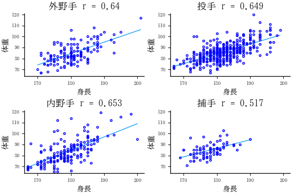

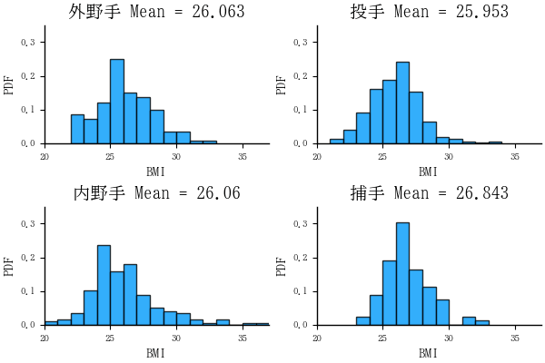
BMI のヒストグラム描画
function distributionofbmi(df; group=df[1, 3])
    bmi = floor.(Int, df[!, :BMI] ./ 0.5) .* 0.5
    res2 = freqtable(bmi)
    plt = histogram(df[!, :BMI], bins=15, alpha=0.8,
        xlims=(20, 37), xlabel="BMI",
        ylims=(0, 0.35), ylabel="PDF", normalize=:pdf,
        tick_direction=:out)
    title!("$group Mean = $(string(round(mean(df[!, :BMI]), digits=3)))")
    plt
end

plt0 = distributionofbmi(df2, group="全選手")
plt1 = distributionofbmi(gdf[1]);
plt2 = distributionofbmi(gdf[2]);
plt3 = distributionofbmi(gdf[3]);
plt4 = distributionofbmi(gdf[4]);
plot(plt1, plt2, plt3, plt4)
savefig("fig2.png")

いくつかわかったこと

• 捕手は比較的小柄な選手が多い。身長は 190 センチ未満，体重は 100 キログラム未満。いわゆる漫画のドカベンタイプ（大男）のイメージではない。しかし，BMI の平均値は 26.843 と最も高いので，小さいがずんぐりしているのかもしれない。
• 身長と体重の相関係数は，捕手が 0.517 と一番低い。内野手，投手，外野手では 0.65 程度である。

Julia に翻訳--239 PISA 2018データを読む，SPSS の .sav ファイル

#==========
Julia の修行をするときに，いろいろなプログラムを書き換えるのは有効な方法だ。
以下のプログラムを Julia に翻訳してみる。

PISA 2018データを読む
https://oku.edu.mie-u.ac.jp/~okumura/python/pisa2018.html

ファイル名: .jl　　関数名:

翻訳するときに書いたメモ

途中で NamedArray のまま処理を進めるようにしたが，データフレームにして transform などを使ってデータ処理をしたほうがわかりやすいかもしれないが，まあいいか。

==========#

#==
>>> import pyreadstat
>>> from time import time
>>> s = time()
df, meta = pyreadstat.read_sav('STU/CY07_MSU_STU_QQQ.sav')
print(time()-s)
# 92.55421423912048 sec.
==#

using StatFiles, DataFrames, CSV
# @time df = DataFrame(load("STU/CY07_MSU_STU_QQQ.sav"))

とてつもなく遅い（4時間ぐらい！！！かかった）
R か Python で読んで，CSV ファイルの保存してから Julia でやるほうがよい。

@time CSV.write("STU/CY07_MSU_STU_QQQ.csv", df) # 255.005749 seconds
@time df = CSV.read("STU/CY07_MSU_STU_QQQ.csv", DataFrame) # 67.728522 seconds。 2回目以降は早くなる 46.337307 seconds
Base.summarysize(df)　# 5,464,156,768 byte
size(df) # (612004, 1119)
first(df, 2)
# 2 rows × 1,119 columns (omitted printing of 1110 columns)
#  CNTRYID CNT CNTSCHID CNTSTUID CYC NatCen STRATUM SUBNATIO OECD
#  Float64 String Float64 Float64 String Int64 String Int64 Float64
# 1 8.0 ALB 800002.0 800251.0 07MS 800 ALB0109 80000 0.0
# 2 8.0 ALB 800002.0 800402.0 07MS 800 ALB0109 80000 0.0
names(df)
# 1119-element Vector{String}:
#  "CNTRYID"
#  "CNT"
#  "CNTSCHID"
#  "CNTSTUID"
#  "CYC"
#  ⋮
#  "SENWT"
#  "VER_DAT"
#  "test"

#> "IC001Q01TA" の回答の度数分布を表示する：

using FreqTables
freqtable(df[!, :IC001Q01TA])
# 4-element Named Vector{Int64}
# Dim1    │
# ────────┼───────
# 1.0     │ 207182
# 2.0     │  50529
# 3.0     │  97676
# missing │ 256617

#> 国名と回答の度数分布

freqtable(df[!, :CNT], df[!, :IC001Q01TA])
# 80×4 Named Matrix{Int64}
# Dim1 ╲ Dim2 │     1.0      2.0      3.0  missing
# ────────────┼───────────────────────────────────
# ALB         │    3940      558     1589      272
# ARE         │       0        0        0    19277
# ARG         │       0        0        0    11975
# AUS         │    6858     2406     2738     2271
# AUT         │    4797      626      972      407
# USA         │    2577      843     1183      235
# VNM         │       0        0        0     5377

#> 日本に限れば

gdf = groupby(df, :CNT)
jpn = gdf[(CNT="JPN",)]
freqtable(jpn[!, :IC001Q01TA])
# 4-element Named Vector{Int64}
# Dim1    │
# ────────┼─────
# 1.0     │ 2200
# 2.0     │ 1790
# 3.0     │ 2029
# missing │   90

#> 国ごとに回答1の割合を求めるには

# クロス集計
tbl = freqtable(df[!, :CNT], df[!, :IC001Q01TA])
# 80×4 Named Matrix{Int64}
# Dim1 ╲ Dim2 │     1.0      2.0      3.0  missing
# ────────────┼───────────────────────────────────
# ALB         │    3940      558     1589      272
# ARE         │       0        0        0    19277
# ARG         │       0        0        0    11975
# ⋮                   ⋮        ⋮        ⋮        ⋮
# USA         │    2577      843     1183      235
# VNM         │       0        0        0     5377

# 全てが missing の国を除く
tbl2 = tbl[((tbl[:, 1] .!= 0) .& (tbl[:, 2] .!= 0) .& (tbl[:, 3] .!= 0)), :]
# 53×4 Named Matrix{Int64}
# Dim1 ╲ Dim2 │     1.0      2.0      3.0  missing
# ────────────┼───────────────────────────────────
# ALB         │    3940      558     1589      272
# AUS         │    6858     2406     2738     2271
# AUT         │    4797      626      972      407
# ⋮                   ⋮        ⋮        ⋮        ⋮
# URY         │    2197      556     1351     1159
# USA         │    2577      843     1183      235

# missing を除いたサンプルサイズ
rowsum = sum(tbl2[:, 1:3], dims=2)
# 53×1 Named Matrix{Int64}
# Dim1 ╲ Dim2 │ sum(Dim2)
# ────────────┼──────────
# ALB         │      6087
# AUS         │     12002
# AUT         │      6395
# ⋮                     ⋮
# URY         │      4104
# USA         │      4603

# 回答1の割合
s = vec(tbl2[:, 1] ./ rowsum)
# 53-element Vector{Float64}:
#  0.647281090849351
#  0.5714047658723546
#  0.7501172791243159
#  ⋮
#  0.5353313840155945
#  0.559852270258527

# 国名取り出し
country = names(tbl2)[1]

# 並べ替え順（R の order()）
o = sortperm(s)

# 3文字略称を日本語名に変換
countryname = CSV.read("countryname.csv", DataFrame);
name = fill("", length(s));
for (i, abb3) in enumerate(country[o])
    j = indexin([abb3], countryname[!, :abb3])[1]
    name[i] = isnothing(j) ? abb3 : countryname[j, :nameJ]
end

# ドットプロット
using Plots
pyplot()
plt = scatter(
 s[o],
 country[o],
 tick_direction=:out,
 size=(500, 700),
 label="")
yticks!(0.5:length(name), name)
savefig("fig.png")