Julia で VolcanoPlot

一部でよく使われている散布図の一種ということで，R で ggplot を使ったり，Python でも書かれたりしているので，Julia でもやって見ようと思う次第。

以下が，特に参考になった。

19.11 Volcano plots
https://biocorecrg.github.io/CRG_RIntroduction/volcano-plots.html

順をおって Julia に書き換えていく。

# The RDS format is used to save a single R object to a file, and to restore it.
# Extract that object in the current session:
# tmp <- readRDS("de_df_for_volcano.rds")

# import Pkg; Pkg.add("RData")
using RData # for load()
tmp = load("de_df_for_volcano.rds"); # read *.rds file

typeof(tmp) # DataFrames.DataFrame
size(tmp)   # (21276, 3)

first(tmp, 5);
#=
5 rows × 3 columns

 gene_symbol log2FoldChange pvalue
 String Float64 Float64⍰
1 Ndufa9 -0.876454 3.38515e-34
2 Rpp21 -0.976487 1.56044e-26
3 Amotl1 -0.758269 2.16481e-24
4 Gm44064 -0.848502 5.12505e-20
5 Hcfc1r1 -0.602129 3.7995e-17
=#

last(tmp, 5);
#=
5 rows × 3 columns

 gene_symbol log2FoldChange pvalue
 String Float64 Float64⍰
1 Ccny 0.0210335 missing
2 Ccne2 -0.00542747 missing
3 Ptk2 -0.00718793 missing
4 Gm26762 -0.0127217 missing
5 Smg1 -0.00845303 missing
=#

# remove rows that contain 'missing' (NA in R) values
# de <- tmp[complete.cases(tmp), ]

using DataFrames
de = dropmissing(tmp);
size(de) # (13421, 3)
first(de, 5);
#=
5 rows × 3 columns

 gene_symbol log2FoldChange pvalue
 String Float64 Float64
1 Ndufa9 -0.876454 3.38515e-34
2 Rpp21 -0.976487 1.56044e-26
3 Amotl1 -0.758269 2.16481e-24
4 Gm44064 -0.848502 5.12505e-20
5 Hcfc1r1 -0.602129 3.7995e-17
=#
tail(de, 5);
#=
5 rows × 3 columns

 gene_symbol log2FoldChange pvalue
 String Float64 Float64
1 Gm28370 -0.0237516 0.999997
2 Shfm1 -0.0267844 0.999997
3 Epc1 0.0161881 0.999997
4 Star -0.0688607 0.999997
5 Gm14137 0.0368722 0.999997
=#

# The basic scatter plot: x is "log2FoldChange", y is "pvalue"
# ggplot(data=de, aes(x=log2FoldChange, y=pvalue)) + geom_point()

using Plots
pyplot(grid=false,
       size=(400, 400), label="")
plt = scatter(de.log2FoldChange, de.pvalue, markerstrokewidth=0,
              alpha=0.4, tick_direction=:out, grid=false,
              xlabel="log2FoldChange", ylabel="pvalue", label="")
savefig("fig1")

ここまでの図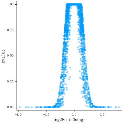

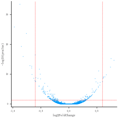
# Convert the p-value into a -log10(p-value)
plt = scatter(de.log2FoldChange, -log10.(de.pvalue),
          markersize=2, markerstrokewidth=0, alpha=0.4,
          tick_direction=:out, tickfontsize=6,
          xlabel="log2FoldChange", ylabel="-log10(pvalue)",
          guidefontsize=8, label="")
# Add vertical lines for log2FoldChange thresholds, and one horizontal line for the p-value threshold
vline!([-0.6, 0.6], color=:red, linewidth=1, linestyle=:dot)
hline!([-log10(0.05)], color=:red, linewidth=1, linestyle=:dot)

# add a column of NAs
# de$diffexpressed <- "NO"
# if log2Foldchange > 0.6 and pvalue < 0.05, set as "UP"
# de$diffexpressed[de$log2FoldChange > 0.6 & de$pvalue < 0.05] <- "UP"
# if log2Foldchange < -0.6 and pvalue < 0.05, set as "DOWN"
# de$diffexpressed[de$log2FoldChange < -0.6 & de$pvalue < 0.05] <- "DOWN"
insertcols!(de, 4, :diffexpressed => "NO");
de.diffexpressed[(de.log2FoldChange .> 0.6) .& (de.pvalue .< 0.05)] .= "UP";
de.diffexpressed[(de.log2FoldChange .< -0.6) .& (de.pvalue .< 0.05)] .= "DOWN";
savefig("fig2.png")

ここまでの図

# Re-plot but this time color the points with "diffexpressed"
# p <- ggplot(data=de, aes(x=log2FoldChange, y=-log10(pvalue), col=diffexpressed)) + geom_point() + theme_minimal()

assigncolor(x) = x == "NO" ? :black : x == "DOWN" ? :blue : :red
plt2 = scatter(de.log2FoldChange, -log10.(de.pvalue),
          color=assigncolor.(de.diffexpressed),
          markersize=3, markerstrokewidth=0, alpha=0.5,
          tick_direction=:out, tickfontsize=6,
          xlabel="log2FoldChange", ylabel="-log10(pvalue)",
          guidefontsize=8, label="")
vline!([-0.6, 0.6], color=:red, linewidth=1, linestyle=:dot)
hline!([-log10(0.05)], color=:red, linewidth=1, linestyle=:dot)
ypos = (maximum(-log10.(de.pvalue))-log10.(0.05)) / 1.5
annotate!(-0.6, ypos, text(" DOWN", 8, :blue, :left))
annotate!( 0.6, ypos, text("UP ",   8, :red,  :right))
savefig("fig3.png")

ここまでの図

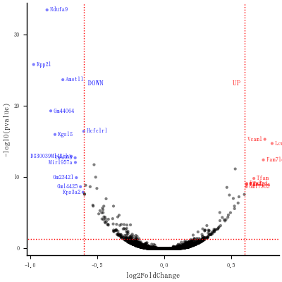
# Now write down the name of genes beside the points...
# Create a new column "delabel" to de, that will contain the name of genes differentially expressed (NA in case they are not)

今までのにプラスして，

for i = 1:size(de, 1)
      x = de[i, :log2FoldChange]
      y = -log10(de[i, :pvalue])
      d = de[i, :diffexpressed]
      if d == "DOWN"
            annotate!(x, y,
                  text(" $(de.gene_symbol[i]) ", 6, assigncolor(d),
                  y > 15 ? :left : :right))
      elseif d == "UP"
            annotate!(x, y,
                  text(" $(de.gene_symbol[i]) ", 6, assigncolor(d),
                  y > 15 ? :right : :left))
      end
end
savefig("fig4.png")

最終の図

ただし，ラベルがグッチャリとしているのは解消できず。

このあと，一般化した関数を提示する予定。